Improved data fitting in 2.5
Continuing the introduction of the new features coming soon with the next release of LabPlot (see the previous blogs here and here), we want to share today some news about the developments we did for the data fitting (linear and non-linear regression analysis) in the last couple of months.
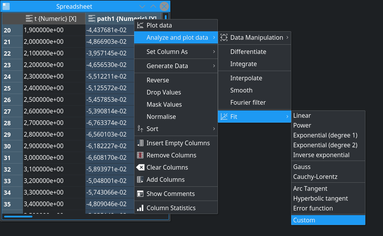
Data fitting, one of the most common and frequently used data analysis tasks, got a lot of improvements. As already mentioned in the previous blog, all analysis functions benefited from the recent general UX improvements. Instead of going through the many manual steps, the final fit result can now be quickly produced via the context menu of the data spreadsheet or directly in the plot in the context menu of the data curve:
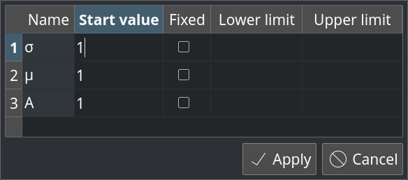
Until now, the fit parameters could in principle take any values allowed by the fit model, which would lead to a reasonable description of the data. However, sometimes the realistic regions for the parameters are known in advance and it is desirable to set some mathematical constrains on them. LabPlot provides now the possibility to define lower and/or upper bounds for the fit parameters and to limit the internal fit algorithm to these regions only. Also, it is possible now to fix parameters to certain already known values:
Some consistency checks were implemented to notify the user about wrong inputs (upper bound is smaller than the lower bound, start value is outside of the bounds, etc.) immediately.
The internal parser for the mathematical expressions learnt to recognize arbitrary user-defined parameters. With this, the fit parameters of custom models are automatically determined and there is no need for the user anymore to explicitly specify the parameter names manually once more when providing the start values and the constraints for them.
To obtain the improved parameter estimators for data where the error in the measurements is not constant across the different data points, fitting with weights is used usually as one of the methods to account for such unequal distributions of errors. Fitting with weights is supported in LabPlot now. Different weighting methods are available to ensure the appropriate level of influence of the different errors on the final estimation of the fit parameters. Furthermore, the errors for both, the x- and y-data points, can be accounted for.
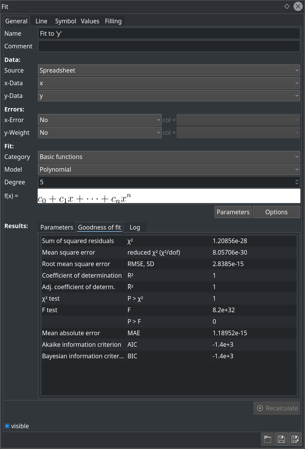
The representation of the fit results was extended. In addition to what was already available in the previous release of LabPlot for the goodness of the fit, new criteria were added like t and p values, the probability that the null hypothesis in the t-test is true, confidence intervals, Akaike- and Bayesian information criteria. The screenshot below shows the current version of the fit dock widget:
Though quite a lot of features are already available in LabPlot in this area, many important and useful features like the support for different fitting algorithms, the subtractions of baseline from a spectrum, etc. need to be implemented. We hope to close the open gaps here very soon in one of the next releases.
[…] [LabPlot] Improved data fitting in 2.5 […]
Since the demise of QtiPlot as a free OS project, I’m following LabPlot development with great interest because I do a lot of data fitting to my own equations (biophysical data). So, any likely release date for v2.5? I mean, roughly: one month from now, four months…
On the other hand, how is the collaboration with SciDavis going? Is it still alive?
Thanks for your attention and, above all, for making LabPlot possible.
sorry for the late reply. I somehow missed your comment. We planned to release 2.5 last December but had to postpone it because of another important feature that needs more time. A blog post on this will come soon. We’ll need one month or so to stabilize everything. So, somewhere in April the next release is to be expected. In the meantime you can try the current version by compiling from the source code if it’s feasible for you. Every feedback and bug reports are welcome and we still have some time to react on them.
There is no collaboration with SciDavis anymore. The two SciDavis developers quitted the collaboration already long time ago. The persons who took over the project on sourceforge couple of years later were not really interested in any kind of collaboration. I’m not sure SciDavis is still alive….
Oh! Sad news regarding SciDavis [collaboration].
In the meantime, I played around with LabPlot 2.4 to see if I could fit some data to a basic non-linear custom equation. What I found out is that, unless your initial guess of the parameter values practically coincides with the real values, the fitting process is not able to find them, which basically renders the non-linear fitting in 2.4 useless in its current incarnation, in my humble opinion.
Will it improve in 2.5?
We did a lot to improve data fitting in 2.5. There are now a lot of pre-defined model and advanced options (fixed & limited parameter, more statistics, x- and y-error, weighting etc.). We also added a lot of tests to make sure it works on any platform.
There are already packages for Windows and Mac to test it. On Linux you should install the latest version from source. It would be great if you could check it out.
Thanks for your efforts. I’m willing to check it out.
Since I’m a gentoo user, I tried to install the latest -9999 version, but the ebuild is unable to find the source code and I already filed the corresponding bug:
https://bugs.gentoo.org/653090
Well, thanks to the amazing Gentoo developers, the bug has been solved in no time!
These are the issues I have found so far:
a) When entering data into a spreedsheet, labplot-2.5.0 does not honor my numeric format setting. Since I’m a Spaniard, I have my KDE 5 configured to enter decimals with a “,”. The thing is, no matter how I enter a decimal number (2,3 or 2.3, for instance), the number is simply ignored after pressing enter, as if I had not entered anything. BUT, if I just enter a number with no decimal places or I use a power, like 23e-1, then I get a correct 2,3 in the cell (yes, lablot 2.5.0 then chooses the comma to show the decimal separator).
b) When I right click on the spreedsheet to plot the data, labplot shows just one of the columns as an option for both axes, i.e., it just shows column number 2 in the drop-down menus to select which data columns are to be plotted for x and y. Later on you can correct that.
c) The non-linear fitting seems to be working OK. For instance, when I fit some enzymatic data to the basic Michaelis-Menten equation, Vm*x/(Km+x), it ocrrectly detects Vm and Km as parameters and is able to find the best fitting values for them.
BUT, there seems to be a bug in the parameter recognition. For instance, if the custom equation is something like this (Lindemann mechanism): k1*k2*x/(km1*x+k2), then k2 is duplicated in the parameters window where you enter their initial guesses and the duplicate k2 is even fitted for and assigned a diferrent value than the “first” k2.
Hope this helps.
The general fitting procedure seems promising and vastly improved. Thanks very much!
Thanks a lot for your feedback!
The last issues with the fit parameters is fixed now. Please pull the new code and try again. I cannot reproduce the second issue…
Can you please create a bug ticket on bugs.kde.org for LabPlot for every open problem you have right now? The discussion about problems is much easier in bugzilla. We’re in the phase of stabilizing the next release 2.5. and every user’s feedback is very welcome. So, simply create bug reports and we will take care of them.
Thanks. I already filed three different bugs.