Performance of data import in LabPlot
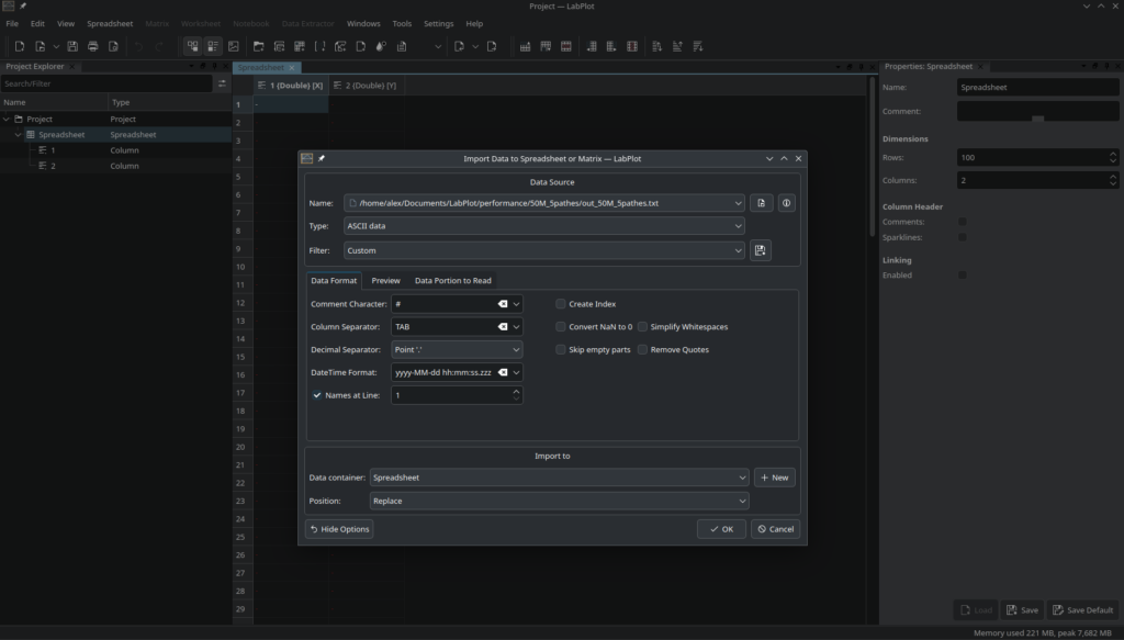
In many cases, importing data into LabPlot for further analysis and visualization is the first step in the application:

LabPlot supports many different formats (CSV, Origin, SAS, Stata, SPSS, MATLAB, SQL, JSON, binary, OpenDocument Spreadsheets (ods), Excel (xlsx), HDF5, MQTT, Binary Logging Format (BLF), FITS, NetCDF, ROOT (CERN), LTspice, Ngspice) and we plan to add support for even more formats in the future. All of these formats have their reasons for existence as well as advantages and disadvantages. However, the performance of reading the data varies greatly between the different formats and also between the different CPU generations. In this post, we’ll show how long it takes to import a given amount of data in four different formats – ASCII/CSV, Binary, HDF5, and netCDF.
This post is not about promoting any of the formats, nor is it about doing very sophisticated measurements with different amounts and types of data and extensive CPU benchmarking. Rather, it’s about what you can (roughly) expect in terms of performance on the new and not so new hardware with the current implementation in LabPlot.
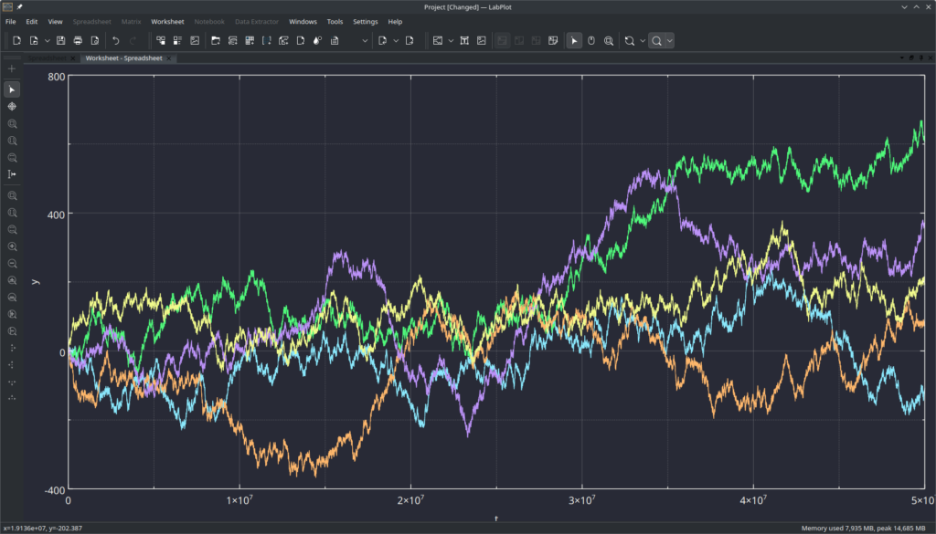
For this exercise, we import the data set with 1 integer column and 5 columns of float values (Brownian motion for 5 “particles”, one integer column for the index) with 50 Millions of rows which results into 300 Millions of numerical values:

We take 6 measurements for each format, ignore the first measurement, which is almost always an outlier due to the disk cache in the kernel and results in faster file reads on subsequent accesses, and calculate the averages:

As expected, the file formats that deal with binary representation internally (Binary, HDF5, NetCDF) provide significantly better performance compared to ASCII, and this difference becomes larger the slower the CPU is. The performance of HDF5 and NetCDF is almost the same because the newer version of NetCDF is based on HDF5.
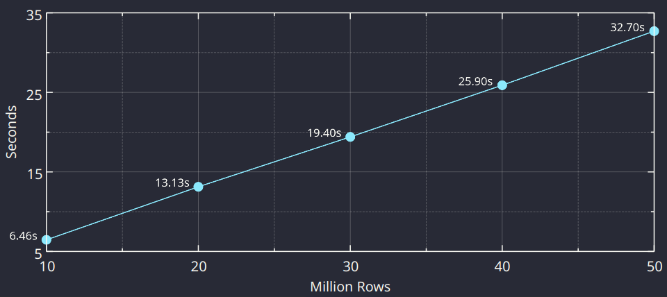
The implementation in the data import code is straightforward. Ignoring for a moment the complexity with the different options affecting the behavior of the parser, different data types and other subleties, once everything is set up it’s just a matter of iterating over the data, parsing it and converting it into the internal structures. The logic inside the loop is fixed, and a linear behavior with respect to the total number of values to read is expected. This expectation is confirmed using the same CPU (we took the fastest CPU from the table above) and varying the total number of rows with the fixed number of columns:

The performance of the import is even more critical when dealing with external data that is frequently modified. In order to provide a smooth visualization in LabPlot for such “live data”, it’s important to optimize all steps involved here, like the import of the new data itself, as well as the recalculation in the algorithms (smoothing, etc.) and in the visualization part. For the next release(s), we’re now working to further optimize the implementation to handle more performance-critical scenarios in the near future. The results of these activities, funded by the NLnet grant, will be the subject of a dedicated post soon.